Introduction
The damped, driven oscillator with two attractive wells has been modelled extensively by Holmes[1], Moon[2], and Li[3]. The governing equation for the system is a fourth-order, partial differential equation. Holmes[1] demonstrates how to reduce it to a second-order, ordinary differential equation. This simplified equation has the form:
where ![]() is the damping coefficient, F is the amplitude
of the driving force,
is the damping coefficient, F is the amplitude
of the driving force, ![]() is the driving frequency. The constants
is the driving frequency. The constants
![]() and
and ![]() are positive constants that determine the height
and width of the of the potential barrier separating the (attractive) wells. In the same paper, Holmes derives a condition
among F,
are positive constants that determine the height
and width of the of the potential barrier separating the (attractive) wells. In the same paper, Holmes derives a condition
among F, ![]() ,
, ![]() ,
,
![]() , and
, and ![]() for the onset
of bifurcations:
for the onset
of bifurcations:
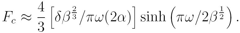
For F greater than Fc chaotic behavior appears. Moon and Holmes[2] have also studied a physical model of the oscillator. The apparatus consisted of a thin, stiff ferrous beam held fixed at one end with the other end placed between two magnets. Without driving and at equilibrium, the free end of the beam rests over one of the magnets. The driving is introduced by shaking the entire apparatus along the line joining the magnets. The experimental results are in close agreement with the numerical results of Holmes. Moon and Li[3,4] have also shown that the boundary between the wells is smooth for F < Fc and fractal for F > Fc.
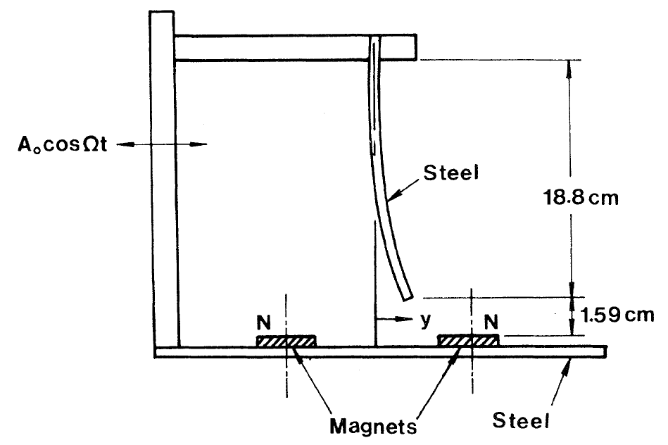
Figure 1.1 Taken from Moon[4]
Methods
We wrote the code in c++ using the algorithms by Kincaid and Cheney [6], and used MathematicaTM for post-processing and visualization.
-
Convergence and Stability
To determine the level of convergence and stability of the algorithms we employed, we utilized the special nature of the seperatrix in the undamped, undriven system since any numerical error would cause the integrator to "fall off" of it. For our tests we started the integrators with the initial condition x = 1 and v = 0, where v is the velocity. More specifically, the branch of the seperatrix we used was the unstable manifold for the saddle-node fixed point at the origin. (A saddle-node fixed point is stable along one direction, i.e. the stable manifold, but unstable along another, i.e. the unstable manifold.) In fact, we chose the constants in the system so that we could use this point for our stability tests. To estimate the error, we used the closest approach distance of the numerical solution from the origin.
-
Numerical Methods
We first looked at using a Runge-Kutta Fourth Order method (referred to as RK4), which has a fifth order truncation error, because we were concerned that the non-linearity of the system would lead to dramatic instabilities in the numerical approximation. As you can clearly see, the RK4 method with a step size of 0.1 "falls inwards" towards the well indicating that the algorithm has an inherint dissipative effect.
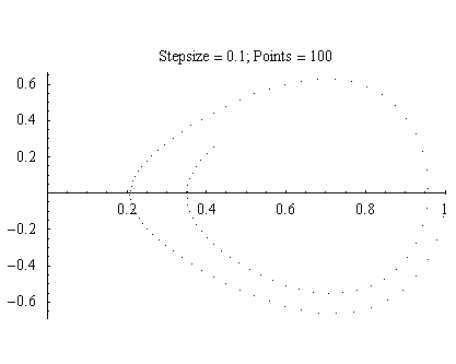
Figure 2.1
Better convergence can be found by increasing the step size, but at significant computional cost.
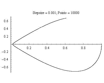
Figure 2.2
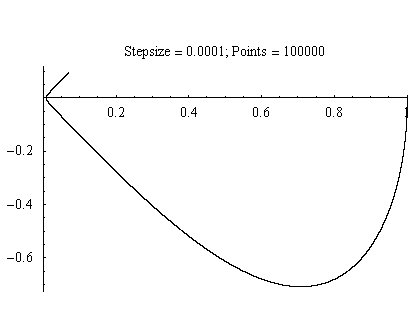
Figure 2.3
The 0.0001 step size comes close to reaching the origin. But, if we zoom in, the closest point is nearly 0.01 units away from the origin.
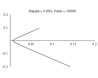
Figure 2.4
So, we decided to see if we could do better using an adaptive Runge-Kutta-Felhberg method (referred to as RKF). The RKF algorithm works by combining two Runge-Kutta methods with different orders. By calculating the differences between the two Runge-Kutta methods, the algorithm generates an estimate of the local error This value is compared to a tolerance from which the point is either accepted or rejected. In either case, in our implementation we update the step size for the next iteration, anyway. These methods tend to be conservative in that the local error is determined via the lower order method, and the solution points returned are those determined by the higher order method.
The RKF method we used combines a fourth and a fifth order method resulting in only 6 function evaluations, where the RK4 method had 4 function evaluations. The routine for adjusting the step size uses the following formula
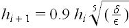
where
 is the tolerance and
 is the estimated error. It is instructive to see this graphically:
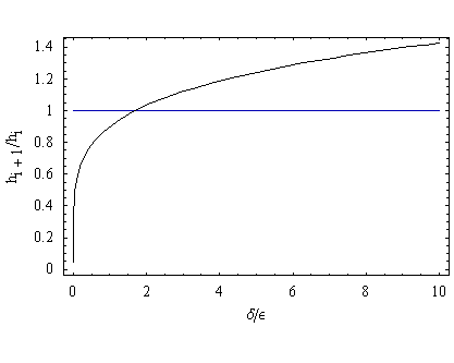
Figure 2.5
The value of the tolerance over the error for which the stepsize remains the same is ~1.7. Above this value, the stepsize is increased slowly. But, below this value the step size is decreased rapidly.
Figure six, below, clearly shows the advantage of using the RKF method over the RK4 method.
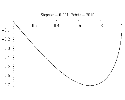
Figure 2.6
With a tolerance of 10-15, the RKF method does not seem to deviate from the seperatrix, and only required a little over 2000 points. (While comparing the point counts is not an accurate method of measuring the differences between the RK4 and the RKF, as the RKF may reject any number of points as unsuitable, it does give a sense of the dramatic speed increase that we noticed when we ran the RKF method.) The magnitude and nature of the error in the algorithm can be found by zooming in on the origin.
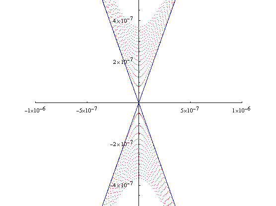
Figure 2.7
The blue lines are the seperatrix. The red dots are the numerical solution which we ran for a long enough time that it completed a little over 15 cycles around the origin. Two things to note here. First, the RKF method appears to add energy into the system, so that as the simulation time increases the numerical solution travels farther and farther away from the origin. Second, with a little over 116,000 points recorded for this run, the error (closest approach distance from the origin) remained below 4*10-7. While this was fantastic, we were still concerned about numerical errors when we turned on the damping and forcing, and we decided to see how far we could push it.
Our original code for the RKF method, used double precision floating point numbers, which according to the sizeof operator in c++, these are 8 times the size of a char variable as far as gcc is concerned. However, a tolerance of 10-15 was the lower limit we could use before we started to run into the limits of machine precision. This necessitated the use of long doubles, which for gcc are 12 times the size of the char variable. After switching over the code to the long doubles, we ran the previous simulation over with a tolerance of 10-18, and here are the results.
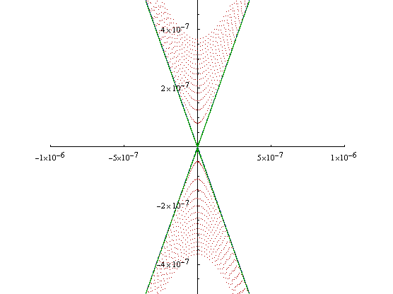
Figure 2.8
The blue lines and the red dots are the same as in Figure 2.7, and the green dots are the 10-18 tolerance solution. As can quickly be seen, the green dots completely cover the seperatrix line at these scales. If we zoom in,
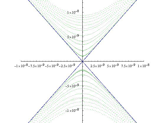
Figure 2.9
the lower tolerance solution is no longer visible whatsoever, and the 10-18 tolerance solution has an error of less than 10-8 after 12 cycles at a cost of a little more than tripling the number of points. Throughout our simulations we used this tolerance level.
Results
We used throughout our simulations a damping coefficient of 0.1 and a driving frequency of 4.
-
Initial Condition Plots
We have seen these types of plots in several places, but without being named. So, we called them initial condition plots. Simply, these types of plots map the system's initial conditions to its position or veloctiy at some future time. They do this by coloring the point in phase space located at the initial condition according to some color function that takes either the system's position or velocity at some specified time. For example, at time zero phase space would look as follows:
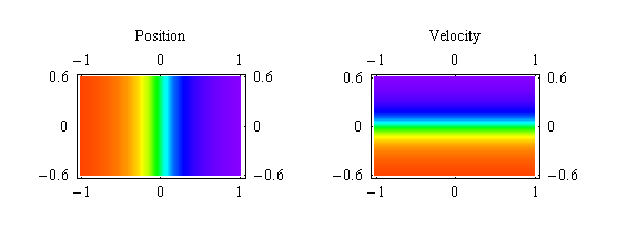
Figure 3.1
As you can readily see, the color functions we employed use the purple end of the spectrum to represent the positive values and the red end of the spectrum to represent the the negative values.
For our simulations, we used a 128 by 128 grid of initial conditions with x between -1 and 1, and v between -0.6 and 0.6. To complete the simulations in time, we opted to run the code on SuperMike by splitting the initial conditions up into 64 seperate regions and allocating a single processor to each region. Figure 3.2 shows the results from this run.
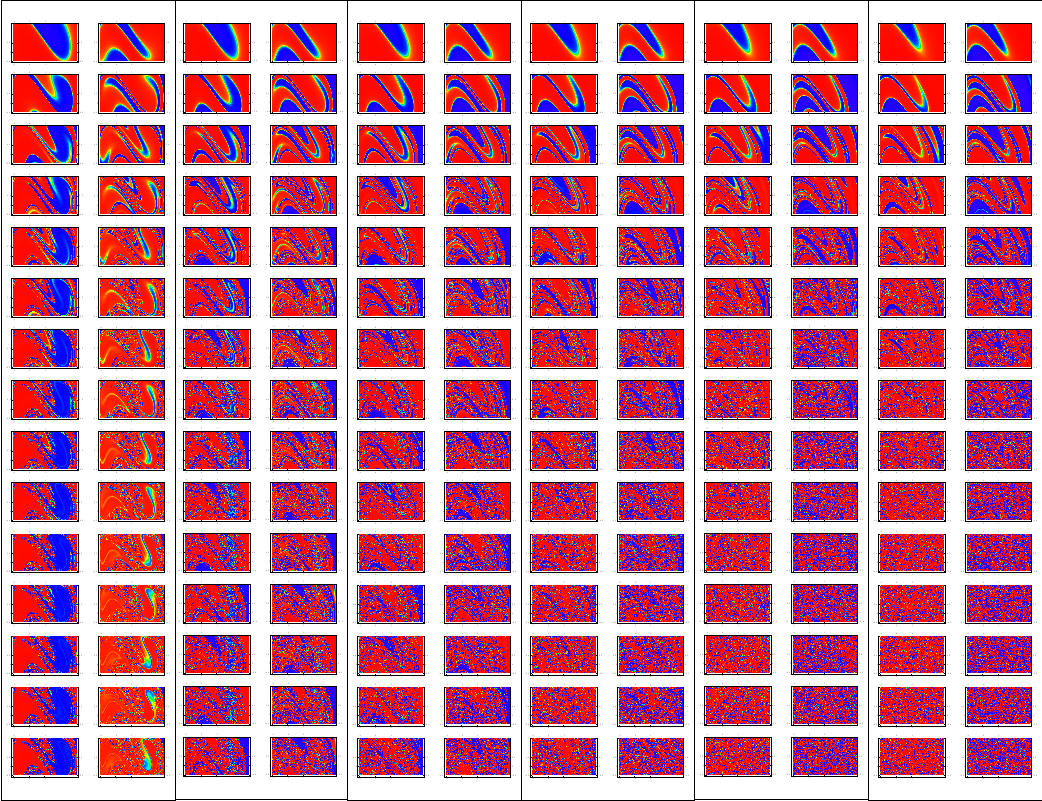
Figure 3.2
Figure 3.2, shows the position and velocity inital condition plots for forcing values of 1, 2, 2.5, 3, 3.5, and 4 for the first 15 drive cycles. The pictures are arranged in position and velocity pairs with increasing force along the horizontal axis, and increasing drive cycle going in integer steps down the vertical axis. A couple of things to note. As you go across the pictures for a particular drive cycle, the features present in the lower forcing cases seem to get squeezed as the force is increased. As you go down through the drive cycles for a single forcing value, the structures in the plots appear to fold in on themselves, and for a forcing of 2 and above they quickly appear to degenerate into noise. This is the fractal basin boundary between the two attractive wells, and it would require an infinite level of resolution to fully resolve.
One way of thinking about the fractal basin boundary is that it is very similar to the real number line. Both irrational and rational numbers have the property of being dense, i.e. between each irrational (rational) number there is another irrational (rational) number, and between each irrational (rational) number there is a rational (irrational) number. This basin boundary is similar to that, as between any two points that end up in the right (left) well there will be at least one point in the left (right) well.
-
Time Series, Phase Space Plots, and Poincare Sections
One can also analyze the results by looking at the time series, phase diagram, and/or Poincare section. The time series shows the position as a function of time. Phase space plots show all possible position-velocity points that the system can access. They give a better picture of the global, long-term behavior of the system. A Poincare section takes a point in phase space once for each period of the driving force. They further reduce the information from a phase space plot, revealing hidden behaviors of the system. These are most effective at distilling out periodic behaviors in the system. For example, a simple periodic system will only have one point in its Poincare section after long period of time. We have added a color element to our Poincare sections to help bring out the time evolution behavior of this system (red is earlier in time, and blue is later in time).
A common reference in the literature is to something called an n-cycle, where n is the number of times a periodic system loops through phase space during a single period. This shows up clearly in a Poincare section as n distinct points, and if you only consider points after the transients have died away, the n points will be the only points in the Poincare section. (See Figure 3.4.2 for an example of a 2-cycle and Figure 3.5.2 for a 3-cycle.) A simple sinusoidal function would be a 1-cycle.
For initial conditions of x = 0.1 and y = 0, we followed the evolution of the system as we increased the forcing from 0.25 to 4 and here is a small selection of our results.
Forcing = 0.25
The first case we examined was for a forcing of 0.25. This is well below any "interesting" behavior. The time series shows early transients damping down to steady oscillation at the driving frequency about the right-hand magnet (attractor) . The phase plot trajectory shows the orbit spiralling down into a limit cycle. The Poincare section shows two points approaching each other. After sufficiently long time the points will merge, again showing damping to the single, driven mode, i.e. it is an example of a 1-cycle. The time series plot confirms this conclusion.
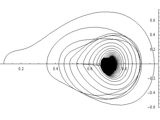
Figure 3.3.1: Phase Space Plot
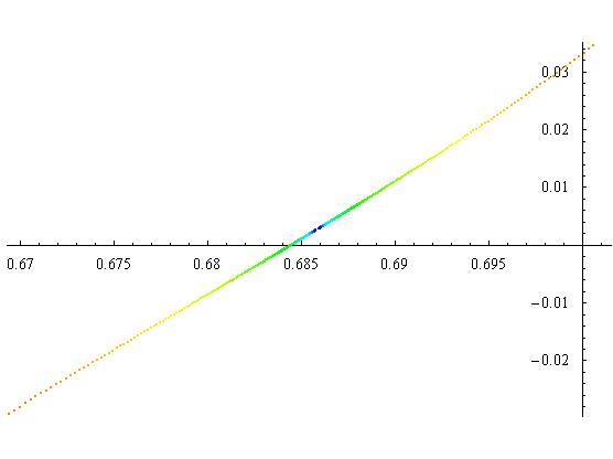
Figure 3.3.2: Poincare Section
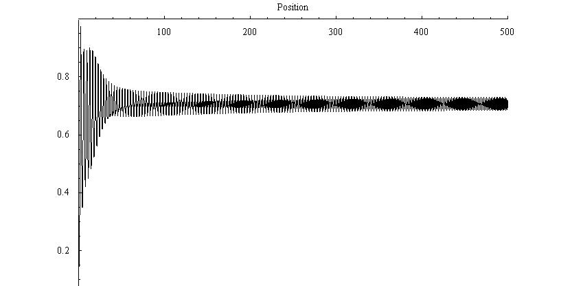
Figure 3.3.3: Time Series plot
Forcing = 1
For a forcing of 1, we start to see some interesting results. The phase space plot shows that the system has to loop around twice before it will return to its starting position, implying that it may be a 2-cycle. This is confirmed by the Poincare section as it has two distinct blue points. The transients are visible as the red and yellow points, and the rest of the spectrum is behind the blue points. After the transients have died off, you can see the beat structure that one would expect in the time series.
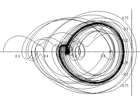
Figure 3.4.1: Phase Space Plot
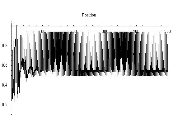
Figure 3.4.3: Time Series plot
Forcing = 2
For a forcing of 2, the system has gone through another bifurcation and is a 3-cycle. The movie is a good way of seeing this behavior.
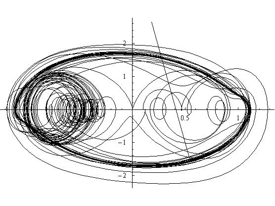
Figure 3.5.1: Phase Space Plot
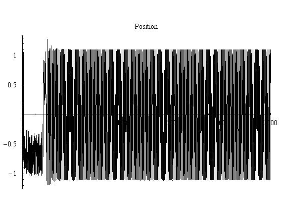
Figure 3.5.3: Time Series plot
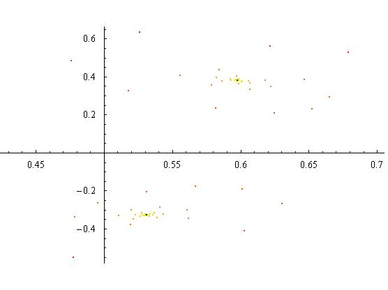
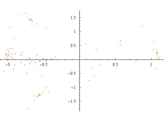
Forcing = 4
A forcing of 4 produces chaos. The phase plot would eventually cover the section of phase space it is currently contained in. Also, the time series shows no repeating structure, and could also be taken as random at first glance. But, the best view of the system is the Poincare section. The structure that is forming in the Poincare section appears to be folded over itself many times and has no simple desription. Also, it clearly can be seen that the later points are spread out across phase space.
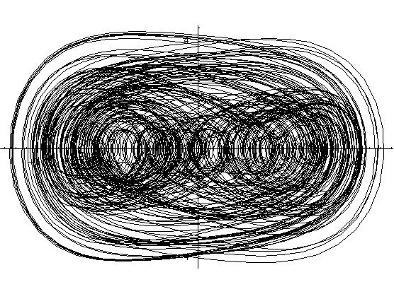
Figure 3.6.2: Phase Space Plot
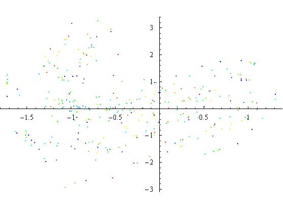
Figure 3.6.2: Poincare Section
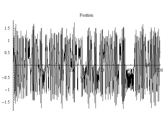
Figure 3.6.3: Time Series plot
-
Movies
We generated movies of the phase space evolutions for forcing values of 0.25, 1, 2, and 4.
References
- P. Holmes, Philos. Trans. Roy. Soc. London A 292 (1979).
- F. Moon and P. Holmes, J. Sound Vib. 62, 275 (1979).
- F. Moon and G.-X. Li, Phys. Rev. Lett. 55, 1439 (1985).
- F. Moon, Phys. Rev. Lett. 53, 962 (1984).
- S. H. Strogatz, Nonlinear Dynamics and Chaos, Studies in Nonlinearity (Addison-Wesley, 1994).
- Kincaid, D. and Cheney, W., Numerical Analysis 2ed., (Brooks/Cole 1996).